MATH ACTIVITY 

USN: 22BSR18013

RAGNEE PRATHAP 

LPP, or linear programming problem, is a technique for determining the best way to solve a collection of parameters that are expressed linearly. We will cover every aspect of linear programming problems in this article, including their kinds, solutions, and applications.

Finding the best solution for a problem that is modelled as a collection of linear relationships is made easier using the linear programming technique. A feasible region, or a region containing all feasible solutions to an LPP, is identified, and the solution is then optimised to obtain the maximum or least function value.

Characteristics of LPP

• The outcomes will depend on the decision variables.
• It is important to quantify the objective function.
• Limitations (restraints) should be expressed mathematically.
• There should be a linear relationship between any two or more variables.
• The variables' values should never be negative or zero.
• Input and output numbers should always be finite and infinite.
  
  

Formulation of LPP

• Determine the deciding factor.
• Compose the objective function.
• List the restrictions.
• List the limitations that are not negative.

Standard Form of LPP

Any Linear Programming Problem can be written as:

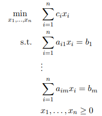
where 

• a_ij and b_j’s are constants, 
• x_i’s are variables (decision variables).

Methods to solve Linear Programming Problems

There are different methods to solve any Linear Programming Problem.

• Graphical Method
• Simplex Method
• North West Corner Method
• Least Square Methods

Graphical Method

Steps for Graphical Method:

• Formulate the LPP.
• Construct the graph and plot all the constraint lines.
• Determine the valid side of each constraint line.
• Identify the feasible solution region.
• Find the optimum points.
• Calculate the coordinates of optimum points.
• Evaluate the objective function at the optimum point.

Example: Solve the given linear programming problem by graphical method.

Max Z = f(x, y) = 3x + 2y

Constraints: 2x + y <= 18

2x + 3y <= 42

3x + y <= 24

x >= 0, y >= 0

Now, let’s plot the graph of the given constraints and find the feasible region.

The above-shaded region (blue color) is the feasible region for the given lpp.

Now, we will find the value of the objective function at the corner points of the feasible region.

From the above table, we got that the objective function obtains its maximum value at (3, 12).

Hence, the maximum value of the objective function f(x,y) = 3x + 2y = 33.

SIMPLEX METHOD

Maximize	Z = f(x,y) = 3x + 2y
subject to:	2x + y ≤ 18
	2x + 3y ≤ 42
	3x + y ≤ 24
	x ≥ 0 , y ≥ 0

1. Change the variables, then normalise the independent terms' signs.

A change is made to the variable naming, establishing the following correspondences:

• x becomes X1
• y becomes X2

There is no need for further action because all restrictions' independent terms are favourable. If not, both sides of the inequality would be multiplied by "-1" (keep in mind that this operation also influences the type of restriction).

2

22. Normalize restrictions.

The inequalities become equations by adding slack, surplus and artificial variables as the following table:

In this case, a slack variable (X3, X4 and X5) is introduced in each of the restrictions of ≤ type, to convert them into equalities, resulting the system of linear equations:

2·X1 + X2 + X3 = 18

2·X1 + 3·X2 + X4 = 42

3·X1 + X2 + X5 = 24

3. Match the objective function to zero.

Z - 3·X1 - 2·X2 - 0·X3 - 0·X4 - 0·X5 = 0

4. Write the initial tableau of Simplex method.

All of the decision variable coefficients from the initial problem are included in the Simplex method's initial tableau, along with the constraints (in rows) and the slack, surplus, and artificial variables added in the second step (arranged in columns with P0 serving as the constant term and Pi serving as the coefficients of the remaining Xi variables). The coefficients for the variables in the base are contained in the Cb column.

The objective function coefficients are in the first row, and the value of the objective function and the decreased costs Zj - Cj are in the last row.

The last row is calculated as follows: Zj = Σ(Cbi·Pj) for i = 1..m, where if j = 0, P0 = bi and C0 = 0, else Pj = aij. Although this is the first tableau of the Simplex method and all Cb are null, so the calculation can simplified, and by this time Zj = -Cj.

                                                                       

5. Stopping condition.

If the goal is to maximise, the stop condition is satisfied when there is no negative value between the discounted costs (P1 columns below) in the last row (the indicator row).

The algorithm then reaches its conclusion because further improvement is not possible. The ideal answer to the issue is the Z value (P0 column).

Another example is where the input variable column of the base has zero or all negative values. This suggests that the issue is widespread and that the best option to solve it is continually being sought after.

If not, the subsequent stages are carried out repeatedly.

6. Choice of the input and output base variables.

The base input variable is chosen first. This is accomplished by selecting the column in Z row whose value is the smallest of all negatives. The variable X1 (P1) in this instance would have a coefficient of -3.

Choose the fundamental variable if there are two or more equal coefficients that satisfy the aforementioned requirement.

The pivot column (shown in green) is the column that contains the input base variable.

The output base variable is established after the input base variable has been received. The choice is based on a straightforward calculation: if both values are strictly positive (greater than zero), divide each independent term (P0 column) by the corresponding value in the pivot column. The row with the lowest score is chosen.

If there is any value less than or equal to zero, this quotient will not be performed. If all values of the pivot column satisfy this condition, the stop condition will be reached and the problem has an unbounded solution (see Simplex method theory).

In this example: 18/2 [=9] , 42/2 [=21] and 24/3 [=8]

The term of the pivot column which led to the lesser positive quotient in the previous division indicates the row of the slack variable leaving the base. In this example, it is X5 (P5), with 3 as coefficient. This row is called pivot row (in green).

If two or more quotients meet the choosing condition (case of tie), other than that basic variable is chosen (wherever possible).

The intersection of pivot column and pivot row marks the pivot value, in this example, 3.

7. Update tableau.

The new coefficients of the tableau are calculated as follows:

• In the pivot row each new value is calculated as:
  New value = Previous value / Pivot
• In the other rows each new value is calculated as:
  New value = Previous value - (Previous value in pivot column * New value in pivot row)

So the pivot is normalized (its value becomes 1), while the other values of the pivot column are canceled (analogous to the Gauss-Jordan method).

8. When checking the stop condition is observed which is not fulfilled since there is one negative value in the last row, -1. So, continue iteration steps 6 and 7 again.

• 6.1. The input base variable is X2 (P2), since it is the variable that corresponds to the column where the coefficient is -1.
• 6.2. To calculate the output base variable, the constant terms P0 column) are divided by the terms of the new pivot column: 2 / 1/3 [=6] , 26 / 7/3 [=78/7] and 8 / 1/3 [=24]. As the lesser positive quotient is 6, the output base variable is X3 (P3).
• 6.3. The new pivot is 1/3.
• 7. Updating the values of tableau again is obtained:

9. Checking again the stop condition reveals that the pivot row has one negative value, -1. It means that optimal solution is not reached yet and we must continue iterating (steps 6 and 7):

• 6.1. The input base variable is X5 (P5), since it is the variable that corresponds to the column where the coefficient is -1.
• 6.2. To calculate the output base variable, the constant terms (P0) are divided by the terms of the new pivot column: 6/(-2) [=-3] , 12/4 [=3] , and 6/1 [=6]. In this iteration, the output base variable is X4 (P4).
• 6.3. The new pivot is 4.
• 7. Updating the values of tableau again is obtained:

10. End of algorithm.

1. It is noted that in the last row, all the coefficients are positive, so the stop condition is fulfilled.

   The optimal solution is given by the val-ue of Z in the constant terms column (P0 column), in the example: 33. In the same column, the point where it reaches is shown, watching the corresponding rows of input decision variables: X1 = 3 and X2 = 12.

   Undoing the name change gives x = 3 and y = 12.

Application of Linear Programming Problem

Numerous industries, including manufacturing, transportation, sports, the stock market, engineering, the energy sector, and machine learning, use linear programming problems. But in this section, we'll talk about some of its practical uses.

Let's say there are 'n' tasks and'm' persons to complete them. Now, delegate the assignment to ensure maximum productivity overall. Setting the smallest cost, the amount of time required for each person, or the most profit will result in the best option. This problem falls under the category of an optimal assignment problem.

Manufacturing industries: These sectors employ lpp models to maximise productivity at the lowest possible cost.

Transport Organisation: Organisations like Rapido, Ola, and Uber employ LPP to optimise delivery routes. These businesses want to make more money while saving time and money on overhead.

Supervised learning applies the principles of linear programming in machine learning.